Mastering ANOVA in Excel: Step-by-Step Guide

Analysis of Variance, commonly known as ANOVA, is a statistical method that allows you to compare means among three or more groups. This technique is pivotal in various fields like agriculture, medicine, social sciences, and business analytics where comparing group means provides insight into complex data sets. In this guide, we'll walk through how to perform ANOVA in Excel, a tool widely accessible to professionals and researchers.
Understanding ANOVA Basics
ANOVA helps determine if there are any statistically significant differences between the means of groups. Here are some key points:
- One-Way ANOVA: Used when you have one independent variable.
- Two-Way ANOVA: Employed when there are two independent variables.
- Between-Subjects and Within-Subjects ANOVA: Between-Subjects compares different groups, while Within-Subjects uses repeated measures from the same subjects.
- Assumptions: Homogeneity of variances, independence of observations, and normality of distribution within groups.
Steps to Perform One-Way ANOVA in Excel
Follow these steps to execute a One-Way ANOVA in Excel:
1. Data Preparation
- Ensure your data is organized with group means in columns or rows, making sure each group’s data is in a separate column or row.
📝 Note: For the best results, keep data clean and consistent. Remove any outliers or errors before proceeding.
2. Accessing ANOVA Tool
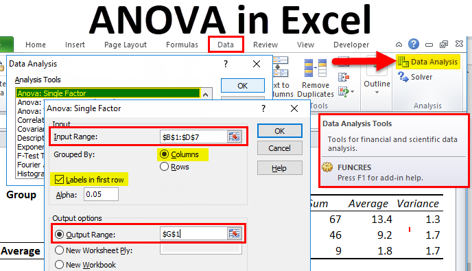
- Go to the ‘Data’ tab on Excel’s Ribbon, click ‘Data Analysis.’ If this option is not available, you will need to add the Analysis ToolPak.
📌 Note: In case 'Data Analysis' is missing, go to 'File' > 'Options' > 'Add-Ins', select 'Analysis ToolPak' and click 'Go'.
3. Inputting Data
- Choose ‘ANOVA: Single Factor’ from the list.
- Input your data range by selecting all data including group labels.
- Ensure the ‘Labels in first row’ checkbox is checked if you’ve included headers.

| Group 1 | Group 2 | Group 3 |
|---|---|---|
| 12 | 15 | 10 |
| 10 | 12 | 16 |
| 13 | 11 | 14 |
4. Running ANOVA
- Choose where you want the output (e.g., new worksheet) and click ‘OK’.
5. Interpreting Results
After running the ANOVA, Excel provides:
- F-ratio: A measure to compare variance between groups to variance within groups.
- P-value: If p < 0.05, reject the null hypothesis (significant difference among groups).
- F crit: The critical value for F at your alpha level; the F-ratio should exceed this for significance.
Important Considerations
When performing ANOVA in Excel, consider:
- Assumptions: Ensure your data meets the assumptions. If not, you might need other tests or transformations.
- Post-hoc Tests: If ANOVA indicates significant differences, use post-hoc tests to find where those differences lie.
- Power Analysis: Before conducting ANOVA, ensure you have adequate power to detect effects.
In conclusion, ANOVA in Excel is a powerful tool for comparing means across multiple groups. By following the steps outlined, you can conduct reliable analyses that provide insights into your data. Whether you're dealing with scientific data, market research, or educational evaluations, understanding and applying ANOVA can offer valuable statistical inference.
What does ANOVA stand for?
+ANOVA stands for Analysis of Variance, which is a statistical method used to test differences between two or more means.
Can Excel handle Two-Way ANOVA?
+Yes, Excel can perform Two-Way ANOVA through the ‘Data Analysis’ tool, but it requires specific setup and interpretation that goes beyond One-Way ANOVA.
What should I do if my data doesn’t meet ANOVA assumptions?
+If assumptions like normality or homogeneity of variances are not met, consider data transformation or using non-parametric alternatives like the Kruskal-Wallis test.


