Modify Excel Pivot Tables with Ease: Quick Guide

Working with data in Microsoft Excel often requires efficient ways to summarize and analyze large datasets. One of the most powerful features in Excel for such tasks is the PivotTable. This guide will walk you through how to modify an Excel PivotTable to get the most out of your data analysis process.

Understanding PivotTables

PivotTables are dynamic tools that allow you to reorganize and summarize selected columns and rows of data in a spreadsheet. They are excellent for:

• Quick data analysis
• Summarizing, sorting, reorganizing, grouping, and presenting data
• Creating dashboards and reports

How to Modify a PivotTable

1. Adding and Removing Fields

Modifying a PivotTable can involve adjusting what data is shown. Here's how:

• To Add Fields: Drag and drop fields from the Field List into the Rows, Columns, Values, or Filters areas. This expands your table to include additional data.
• To Remove Fields: Click the field in the area you wish to remove it from, and then drag it back to the Field List or right-click and select 'Remove Field'.

2. Changing Field Settings

Field settings give you control over how data is displayed:

• Summary Functions: Right-click a value field in the PivotTable, select 'Value Field Settings', and choose a different summary function like 'Sum', 'Count', 'Average', etc.
• Number Formatting: From the 'Value Field Settings' dialog, click on 'Number Format' to apply standard Excel number formatting.

3. Grouping Data

Grouping allows for hierarchical categorization:

• Manual Grouping: Right-click the cell you want to group, choose 'Group', and decide the interval or levels you want to group by.
• Automatic Grouping: Excel can automatically group date/time fields or numeric fields. Simply select the field and go to the 'Analyze' tab, then 'Group Selection'.

🔍 Note: Grouping can also apply to non-numeric data by selecting a range of values manually.

4. Filtering Data

PivotTables provide powerful filtering options:

• Report Filter: Place fields into the ‘Filters’ area to filter the entire table based on a field’s criteria.
• Slicer Filters: Use slicers for interactive filtering. From the ‘PivotTable Analyze’ tab, select ‘Insert Slicer’.
• Label and Value Filters: You can apply more specific filters under row or column labels by right-clicking and selecting ‘Filter’.

5. Layout and Formatting

The layout and visual appearance of a PivotTable can significantly affect data interpretation:

• Compact vs. Tabular Layout: Change this in the ‘Design’ tab under ‘Report Layout’.
• Field Header Styles: Choose from different styles to make headers stand out.
• Band Rows: Enable or disable alternating row colors for better readability.

6. Refreshing Data

Keeping your PivotTable up-to-date with the latest changes in your source data is essential:

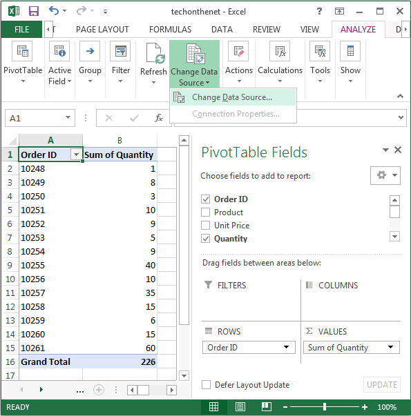
• To refresh manually, click ‘Refresh’ in the ‘PivotTable Analyze’ tab.
• To automatically refresh when the workbook opens, go to the ‘PivotTable Options’ dialog, and select ‘Refresh data when opening the file’.

Modifying your PivotTable in Excel is a game-changer when it comes to data analysis. Whether you're tweaking settings for precision, enhancing your data presentation, or ensuring your data reflects real-time updates, these tips will help you master the PivotTable's capabilities. Your efficiency in data management and presentation will see a marked improvement, making complex data comprehensible and actionable.

FAQ Section