5 Simple Steps to Calculate Sharpe Ratio in Excel

Calculating the Sharpe Ratio is an essential step for investors looking to measure the risk-adjusted return of an investment portfolio. Developed by Nobel laureate William F. Sharpe, this ratio helps in understanding how much excess return you receive for the extra volatility that you endure for holding a riskier asset. Here, we'll dive into how you can easily compute the Sharpe Ratio using Microsoft Excel in just five straightforward steps.
Step 1: Collect and Organize Your Data
Before you can calculate the Sharpe Ratio, you need historical data:
- Historical Returns: Gather the past returns of the investment portfolio or asset you’re analyzing. Ensure these returns are consistent, whether they are monthly, daily, or annual.
- Risk-Free Rate: Obtain the risk-free rate for the same period as your returns. Common proxies for the risk-free rate include the yield of a three-month U.S. Treasury bill, but the choice can vary based on your country and investment timeframe.
To organize:

| Date | Return | Risk-Free Rate |
|---|---|---|
| 01-Jan-2023 | 0.05% | 0.01% |
| 01-Feb-2023 | -0.02% | 0.01% |
📌 Note: Ensure your returns and risk-free rates are in the same time period for accurate comparison.
Step 2: Calculate Excess Returns
The Sharpe Ratio hinges on the idea of “excess returns,” which are the returns from the investment over and above the risk-free rate. Here’s how you compute it in Excel:
- In a new column, subtract the risk-free rate from each return to get the excess returns.
- Use a formula like this:
=B2-C2where B2 is the return for the first period and C2 is the risk-free rate for that period.
Step 3: Compute the Average Excess Return
Next, calculate the average of these excess returns:
- Excel Function:
=AVERAGE(Excess_Returns_Range)
🔍 Note: The average excess return is your mean return above what you could have earned from a risk-free asset.
Step 4: Calculate the Standard Deviation of Excess Returns
Volatility, in this case, is measured by the standard deviation of excess returns:
- Use the Excel function:
=STDEV(Excess_Returns_Range)
Step 5: Compute the Sharpe Ratio
With the average excess return and the standard deviation, you’re now ready to calculate the Sharpe Ratio:
- Sharpe Ratio Formula:
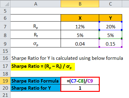
Sharpe Ratio = Average Excess Return / Standard Deviation of Excess Returns - In Excel:
=D13/E13where D13 is the average excess return and E13 is the standard deviation of excess returns.
📘 Note: A higher Sharpe Ratio indicates better risk-adjusted performance, meaning more return for the risk taken.
Summing up, calculating the Sharpe Ratio in Excel is not only practical but also invaluable for investors. It provides a quantitative measure of how well an investment's returns compensate for the level of risk taken. By using Excel, you can efficiently compute this ratio, enabling you to make data-driven investment decisions. Remember that while the Sharpe Ratio is a useful tool, it has its limitations, particularly when returns are not normally distributed. However, when used in conjunction with other metrics, it can offer profound insights into your investment choices.
Why do we use excess returns in Sharpe Ratio?
+Excess returns in the Sharpe Ratio calculation allow us to see how much better an investment performs than a risk-free investment, providing a clear picture of risk-adjusted return.
Can I calculate Sharpe Ratio for different time periods?
+Yes, the Sharpe Ratio can be calculated for any consistent time period. Just ensure that the risk-free rate aligns with the period of returns you are using.
Is a higher Sharpe Ratio always better?
+Generally, yes. A higher Sharpe Ratio indicates better risk-adjusted returns. However, if returns are not normally distributed or if the portfolio is not well-diversified, the interpretation can be less straightforward.


