5 Ways to Alternate Row Colors in Excel

The versatility of Microsoft Excel extends beyond simple calculations, offering various tools for improving both the aesthetics and functionality of spreadsheets. One visually appealing feature is the alternate row colors which significantly enhances the readability of data by making each row visually distinct from its neighbors. This technique is not just about making your data look good; it also reduces errors when interpreting large volumes of information. In this post, we'll explore five different methods to alternate row colors in Excel, ensuring your spreadsheets stand out.

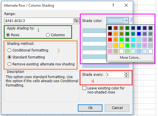
Method 1: Using Excel’s Conditional Formatting

Conditional formatting in Excel is a powerful tool that allows for the application of formatting based on specified rules or conditions. Here’s how you can use it to alternate row colors:

• Select the entire dataset or the range you want to format.
• Navigate to the Home tab, click on Conditional Formatting, then New Rule.
• Choose Use a formula to determine which cells to format.
• Enter the formula =MOD(ROW(),2)=0 to format even rows or =MOD(ROW(),2)=1 for odd rows.
• Click on Format, choose your desired colors, and press OK twice to apply.

⚠️ Note: This method uses dynamic formulas which means the color will adapt if rows are added or removed.

Method 2: Applying Table Styles

Excel’s built-in Table feature can apply alternate row colors with just a few clicks:

• Select your data range or create a table by clicking anywhere in your data and using Insert Table from the Insert tab.
• Once the table is created, go to Table Tools Design under Table Styles.
• Choose from a variety of styles that automatically include alternating row colors.

Method 3: Using VBA

For those who are comfortable with Visual Basic for Applications (VBA), here’s a script to automate the process:

Sub AlternateRowColors()
    Dim rng As Range
    Set rng = Range(“A1:Z100”) ‘ Change this range to fit your data
    rng.Interior.Pattern = xlNone
    Dim i As Integer
    For i = 1 To rng.Rows.Count Step 2
        rng.Rows(i).Interior.Color = RGB(211, 211, 211)
    Next i
    For i = 2 To rng.Rows.Count Step 2
        rng.Rows(i).Interior.Color = RGB(240, 240, 240)
    Next i
End Sub

• Open the VBA editor with Alt + F11, insert a new module, and paste the above code.
• Run the macro by selecting Macros from the Developer tab or pressing Alt + F8.

Method 4: Manual Formatting

Manual formatting can be time-consuming but offers full control:

• Select all rows except the first one by clicking on the row number header, then Shift + Click on the last row number.
• Change the Fill Color in the Home tab.
• Select all odd-numbered rows to apply a different color.

💡 Note: This method is best for small datasets or when precise control over color selection is required.

Method 5: Using a Custom Formula in Conditional Formatting

This method allows for more specific row coloring:

• Follow the initial steps of Method 1 but use a custom formula like =MOD(ROW(),3)=1 for a three-color pattern.
• Set up multiple rules to create various color patterns.

Additional Tips for Enhancing Your Spreadsheet

• Use Banded Columns: Similar to alternating rows, banded columns can be applied using conditional formatting or table styles.
• Keyboard Shortcuts: Master Excel’s shortcuts to speed up formatting tasks. For example, Ctrl + 1 opens the Format Cells dialog.
• Dynamic Ranges: Use named ranges to make formatting formulas dynamic, automatically adjusting as data changes.

In closing, alternating row colors in Excel not only adds a professional touch to your spreadsheets but also significantly aids in data readability and error reduction. Each method discussed here provides different benefits, whether it’s the automation through VBA, the simplicity of table styles, or the flexibility of conditional formatting. Experiment with these techniques to find which suits your needs best, and remember that a well-formatted spreadsheet can communicate information more effectively.